When you examine some of the images listed below,
if you are able to freeze the display mid-course by right-clicking with the mouse,
you may be able to see what overlaps look like before they are replaced by wedges.
(Pointed tiling (1,1,0)P-8 is a good example.
After the image is displayed, toggle between zoom up and zoom down.)
Recall (from § 3.4) that the components σk(j) (j = 1, 2, …, ⌊ n ⁄ 2 ⌋)
of the signature σk
of the kth stage of the tiling are defined as follows:
In either the left or right half of a [horizontally oriented] beadstring of the kth necklace,
σk(j)
is the number of boundary edges with projected length sin jπ/n
on the mirror edge that bisects the beadstring.
Accompanying each of the figures below is a list of signatures for the first few stages of the tiling.
The linear expansion ratio fn is equal to three
for even n tilings and to 1 + 2 cos π ⁄ n for odd n tilings (cf. Fig C3.1.2).
A necessary condition for the existence of blunt RPn tilings
is that tan π/n can be expressed as a linear combination,
with integer coefficients, of sines of integer multiples of π/n (cf. § C3.4).
This requirement is met by odd n but not by even n.
Hence there are no blunt RPn tilings for even n.
For the 'crystallographic integers' n = 2, 3, 4, and 6,
RPn tilings are found to have translation symmetry.
The RP3 tiling in Fig. C3.13.1 immediately below
has translation symmetry if the coloring is ignored.
In this tiling (and also in some of the other figures), mirror edges are shown as faint line segments
superimposed on necklace beadstrings.
For those illustrations in which mirror edges are not drawn and necklaces are not distinguished by color,
necklaces may be recognized by working toward the interior from the outermost necklace
(which is easy to recognize because it is incident at the pattern boundary).
In most of the schematic diagrams like the one at the right in Fig. C3.13.1,
gaps are green and overlaps are red (cf. § C3.1) .
Fig. C3.13.1
RP3
n = 3
f3 = 2
σ1 = (2)P
σ2 = (4)P
σ3 = (8)P
σ4 = (16)P
four stages
p3m1
pdf version
Fig. C3.13.2
RP4
n = 4
f4 = 3
σ1 = (1,1)P
σ1 = (3,3)P
σ1 = (9,9)P
three stages
p4m
pdf version
Fig. C3.13.3
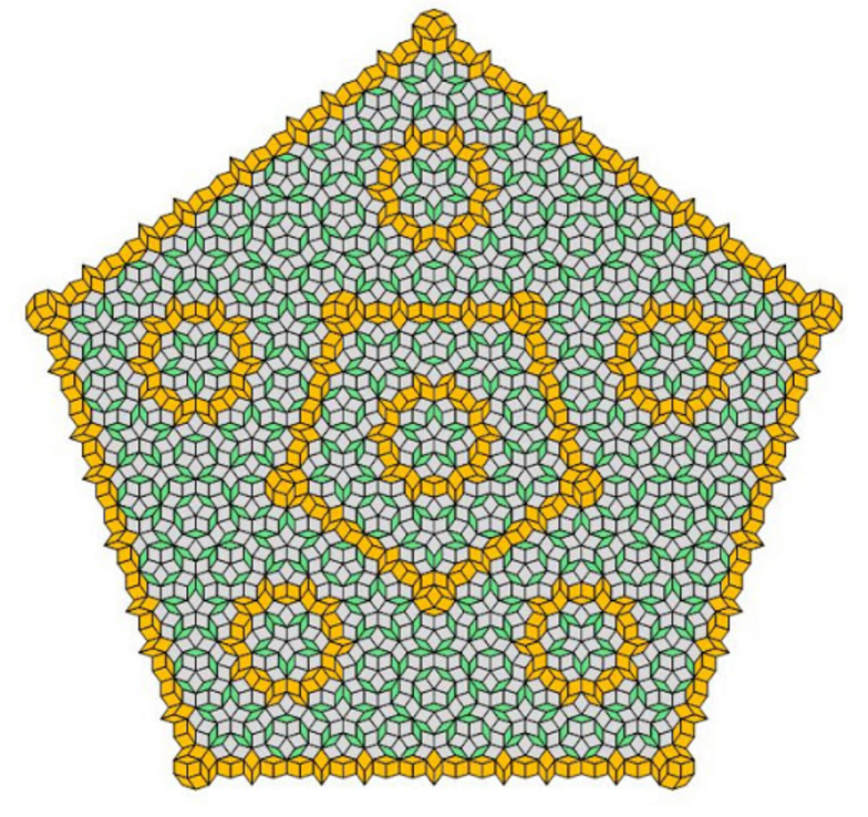
RP5
n = 5
f5 = 1 + φ (≅ 2.618)
σ1 = (1,2)P
σ2 = (3,5)P
σ3 = (8,13)P
three stages
d5
pdf version
.png)
Fig. C3.13.4
RP5
n = 5
f5 = 1 + φ (≅ 2.618)
σ1 = (1,2)B
σ2 = (3,5)B
σ3 = (8,13)B
three stages
d5
pdf version
P.gif)
Fig. C3.13.5
RP6
n = 6
f6 = 3
σ1 = (1,3,1)P
σ2 = (3,9,3)P
σ3 = (9,27,9)P
three stages
p6m
pdf version
P.gif)
Fig. C3.13.6
RP6
n = 6
f6 = 3
σ1 = (2,3,2)P
σ2 = (6,9,6)P
σ3 = (18,27,18)P
three stages
p6m
pdf version
Fig. C3.13.7
RP8
n = 8
f8 = 3
σ1 = (0,2,1,1))P
σ2 = (0,6,3,3))P
σ3 = (0,18,9,9))P
two stages
p8m
pdf version
Fig. C3.13.8
RP9
n = 9
f9 ≅ 2.879
Applying the expansion matrix
E4, with δ9 = (-1,1,1,-1)
(cf. § C3.4), to the intial signature
σ1 = (0,0,1,2)B
to obtain subsequent signatures yields
σ2 = (1,1,3,5)B
and
σ3 = (3,5,9,13)B,
but the second signature here is
σ2 = (2,2,3,4)B,
not (1,1,3,5)B.
Because of the identity
sinπ ⁄ 9 + sin2π ⁄ 9 = sin4π ⁄ 9,
these two different values for σ2 define beadstrings of the same length.
(There is a similar degeneracy for every odd n that is composite.)
two stages
d9
pdf version
C3.14 Gallery of RPn∗ tilings
A necessary condition for the existence of blunt
RPn∗ tilings
is that tan π/n can be expressed as a linear combination,
with integer coefficients, of sines of integer multiples of π/n (cf. § C3.4).
This requirement is met by odd n but not by even n.
Hence there are no blunt RPn∗ tilings for even n.
But if n is equal to twice an odd integer and the prototiles of the tiling
are restricted to the rhombs of SRIn ⁄ 2,
then a blunt tiling is possible.
If n is equal to twice an odd integer, the rhombs that are bisected by radial
lines of reflection to corners of the tiling are oriented oppositely to those that are
bisected by radial lines of reflection to edge midpoints of the tiling (cf. Figs.
C3.14.2, C3.14.3, C3.14.10, and C3.14.14).
Fig. C3.14.1
RP4∗
n = 4
Has one prototile — ρ2— of the two —
ρ1, ρ2 — in SRI4
f2(2) = 3
σ1 = (0,1)P
σ2 = (0,3)P
σ3 = (0,9)P
three stages
p4m
pdf version
The [degenerate] beadstrings and their associated mirror edges are identical in this example.
Fig. C3.14.2
RP6∗
n = 6
Has one prototile — ρ2 — of the three —
ρ1, ρ2, ρ3 — in SRI6
f2(3) = 3
σ1 = (0,1,0)P
σ2 = (0,3,0)P
σ3 = (0,9,0)P
three stages
p6m
pdf version
Fig. C3.14.3
RP6∗
n = 6
Has one prototile — ρ2 — of the three —
ρ1, ρ2, ρ3 — in SRI6
f6 = 3
σ1 = (0,1,0)P
σ2 = (0,3,0)P
σ3 = (0,9,0)P
three stages
p6m
pdf version
Fig. C3.14.4
RP8∗
n = 8
Has two prototiles — ρ2, ρ4 — of the four —
ρ1, ρ2, ρ3, ρ4 — in SRI8
f2(4) = 3
σ1 = (0,1,0,0)P
σ2 = (0,3,0,0)P
σ3 = (0,9,0,0)P
three stages
d8
(1,0)P-1
Fig. C3.14.5
RP8∗
n = 8
Has two prototiles — ρ2, ρ4 — of the four —
ρ1, ρ2, ρ3, ρ4 — in SRI8
f2(4) = 3
σ1 = (0,1,0,0)P
σ2 = (0,3,0,0)P
σ3 = (0,9,0,0)P
three stages
d8
(1,0)P-2
Fig. C3.14.6
RP8∗
n = 8
Has two prototiles — ρ2, ρ4 — of the four —
ρ1, ρ2, ρ3, ρ4 — in SRI8
f2(4) = 3
σ1 = (0,1,0,0)P
σ2 = (0,3,0,0)P
σ3 = (0,9,0,0)P
three stages
d8
(1,0)P-3
Fig. C3.14.7
RP8∗
n = 8
Has two prototiles — ρ2, ρ4 — of the four —
ρ1, ρ2, ρ3, ρ4 — in SRI8
f2(4) = 3
σ1 = (0,1,0,0)P
σ2 = (0,3,0,0)P
σ3 = (0,9,0,0)P
three stages
d8
pdf version
Fig. C3.14.8
RP8∗
n = 8
Has two prototiles — ρ2, ρ4 — of the four —
ρ1, ρ2, ρ3, ρ4 — in SRI8
f2(4) = 3
σ1 = (0,0,1,0)P
σ2 = (0,0,3,0)P
σ3 = (0,0,9,0)P
three stages
d8
pdf version
This tiling bears a slight resemblance to the 1977-1982
'Ammann-Beenker tiling'
illustrated in the
Tiling Encyclopedia
of Dirk Frettlöh and Edmund Harriss.
That tiling, unlike this one, is the dual of a de Bruijn multigrid.
Fig. C3.14.9
RP10∗
n = 10
Has two prototiles — ρ2, ρ4 — of the five —
ρ1, ρ2, ρ3,
ρ4, ρ5 — in SRI10
f2(4) = 3
σ1 = (0,1,0,0,0)P
σ2 = (0,3,0,0,0)P
σ3 = (0,9,0,0,0)P
three stages
d10
pdf version
Fig. C3.14.10
RP10∗
n = 10
Has two prototiles — ρ2, ρ4 — of the five —
ρ1, ρ2, ρ3,
ρ4, ρ5 — in SRI10
f2(5) = 3
σ1 = (0,0,1,0,0)P
σ2 = (2,0,1,0,1)P
σ3 = (4,0,5,0,2)P
three stages
d10
pdf version
Fig. C3.14.11
RP12∗
n = 12
Has two prototiles — ρ2, ρ4 — of the six —
ρ1, ρ2, ρ3,
ρ4, ρ5, ρ6 — in SRI12
f2(6) = 3
σ1 = (0,1,0,0,0,0)P
σ2 = (0,3,0,0,0,0)P
σ3 = (0,9,0,0,0,0)P
three stages
d12
pdf version
Fig. C3.14.12
RP12∗
n = 12
Has three prototiles — ρ2, ρ4, ρ6 — of the six —
ρ1, ρ2, ρ3,
ρ4, ρ5, ρ6 — in SRI12
f2(6) = 3
σ1 = (0,0,1,0,0,0)P
σ2 = (0,0,3,0,0,0)P
σ3 = (0,0,9,0,0,0)P
three stages
d12
pdf version
Fig. C3.14.13
RP14∗
n = 14
Has two prototiles — ρ2, ρ4 — of the seven —
ρ1, ρ2, ρ3,
ρ4, ρ5, ρ6, ρ7 — in SRI14
f2(7) = 3
σ1 = (0,1,0,0,0,0,0)P
σ2 = (0,3,0,0,0,0,0)P
σ3 = (0,9,0,0,0,0,0)P
three stages
d14
pdf version
 Fig. C3.14.14
RP14 tiling
n = 14
Has three prototiles — ρ2, ρ4, ρ6 — of the seven —
ρ1, ρ2, ρ3,
ρ4, ρ5, ρ6, ρ7 — in SRI14
f2(7) = 3
σ1 = (0,0,0,0,0,1,0)P
σ2 = (0,0,0,0,0,3,0)P
σ3 = (0,0,0,0,0,9,0)P
three stages
d14
pdf version
pdf version of modified tiling
Fig. C3.14.15
RP16∗
n = 16
Has two prototiles — ρ2, ρ4 — of the eight —
ρ1, ρ2, ρ3,
ρ4, ρ5, ρ6,
ρ7, ρ8 — in SRI16
f2(8) = 3
σ1 = (0,1,0,0,0,0,0,0)P
σ2 = (0,3,0,0,0,0,0,0)P
σ3 = (0,9,0,0,0,0,0,0)P
three stages
d16
pdf version
C3.15 Some history
In his legendary 1977 essay, Martin Gardner introduced
Penrose tilings in his Scientific American column,
Mathematical Recreations.
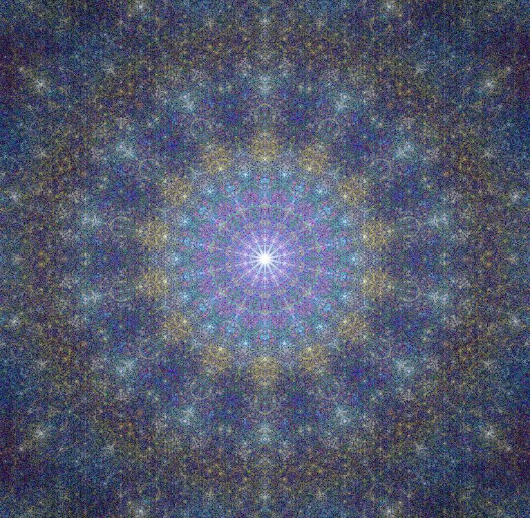
SUN and
STAR
show the central regions of the two d5-symmetric Penrose tilings.
(These images were derived here as duals of
de Bruijn pentagrids.)
In 1981, Nicolaas G. de Bruijn proved that the dual of
every regular pentagrid that satisfies a simple
restriction on the translational shifts γj of the five grids of
the pentagrid is identical to a Penrose tiling
created by arranging rhombs constrained by Penrose's matching rules.
In 1977, after studying Gardner's article, I persuaded a few students
to join me in the study of Penrose tilings.
I ordered steel-rule dies for cutting kites, darts,
and long and short bow-ties from
color-printed cardstock, and we soon amassed a large supply of die-cut tiles.
I decided to focus on the three special Penrose tilings:
SUN (d5 symmetry),
STAR (d5 symmetry),
and
CARTWHEEL (Γ = 0)
When I examined the image of the CARTWHEEL tiling,
I noticed that each of its ten triangular sectors contains
an infinite alternating sequence of successively larger replicas of the central portion
of the SUN or the STAR.
I also observed, but did not prove, that for any two consecutive replicas in this sequence,
the distance from the center of the tiling to the center of the
replica increases by a multiplicative factor equal to the golden ratio.
Looking at the growth outward from the center of the SUN and STAR, I noticed an apparently
recursive structure, which is described below.
I tried unsuccessfully to prove that this recursion continues
beyond its first few iterations.
In the April 1978 Notices of the American Mathematical Society
I published a preliminary report on this topic, although I failed to state that
I had not actually proved anything!
In late 1978,
I welcomed two surprise visitors at my home:
Hank Saxe and Cynthia Patterson, ceramic artists extraordinaire
from Taos, New Mexico.
Hank had been my student and close friend at CalArts several years earlier.
I insisted on holding my two guests (and their golden retriever)
hostage until they agreed to
consider designing and making Penrose patterns from ceramic tiles.
I knew that Hank was expert in the production of colored ceramic glazes,
and I was convinced that together Hank and Cynthia would produce spectacular
works of mathematical art. They didn't disappoint me.
They quickly obtained permission from Roger Penrose to make ceramic versions of his tilings,
and you can see samples of their work on their
website .
In 1979, I encouraged my students to make a 24' x 24' CARTWHEEL tiling by gluing colored paper
rhombs (2 cm. edgelength) onto thirty-six 4' x 4' sheets of masonite. We planned to use the panels
for a traveling Penrose exhibit at Illinois high schools.
When the project was still unfinished at the end of the semester,
we stored the panels in our department building.
Unfortunately, the panels — and other property
stored in the building — mysteriously disappeared during the end-of-semester break,
and work on the project was never resumed.
In those days, I hadn't yet heard of Robert Ammann's work on
aperiodic tilings. It wasn't until 1981 that Nicolaas de Bruijn published his
pair of ground-breaking monographs explaining the
connection between multigrids and Penrose tilings.
(At a Cincinnati AMS meeting soon afterward, David Klarner invited me to spend the evening
with him and his friend de Bruijn, who graciously gave me
copies of his multigrid monographs.)
Now for the first time it became possible to construct Penrose tilings
without having to proceed step-by-step, following matching rules
and hoping you wouldn't end up at an impasse and have to backtrack.
Until de Bruijn's breakthrough, matching rules were the principal device
for forcing aperiodicity.
I also benefited from reading the early articles by the physicist Paul Steinhardt and his students.
This was still several years
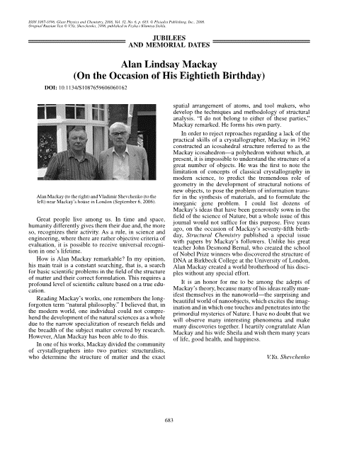
before Shechtman and his colleagues at NIST astonished the world by discovering three-dimensional quasicrystals,
confirming the earlier expectations of Roger Penrose and Alan Mackay (and perhaps nobody else!).
I naively wondered whether one could find a set of matching rules
for tilings by rhombs for n = 7 that would
also force aperiodicity, i.e., allow only non-periodic tilings.
I tried everything I could think of,
but nothing worked. It was only later that I learned that such matching rules
had been proved impossible for n = 7. I was intrigued by
tilings by the three rhombs of SRI7, but
I recognized that tilings by those rhombs — or
any other non-Penrose rhombs — lack the special
charm of authentic Penrose tilings based on the magic number five.
Detour into rhombic rosettes, ROMBIX, and other things
One day in December 1979 I suddenly decided to invent a
new tiling puzzle, by somehow marrying the idea of a polyomino
(the brainchild of Sol Golomb) with the idea of tiling
a regular 2n-gon by
a set of n(n − 1)/2 rhombs, as described by Donald Coxeter.
I decided to experiment by constructing a twin,
in every possible edge-to-edge configuration, from
every possible pair of rhombs in Coxeter's set
of n(n − 1)/2 rhombs.
When I tested this idea for every n ≤ 10, I
was startled to discover that so long as one adds exactly
one specimen of each single rhomb ('keystone') to the collection of twins,
the combined area of all the pieces is precisely equal to that of the regular 2n-gon.
I quickly proved that this holds for all integer n ≥ 3.
I found that I was able to tile the interior of the regular 2n-gon
with some arrangement of the pieces of every set of order n ≤ 12.
Of course it took a lot longer for the larger values of n.
At first I called the puzzle 'CYCLOTOME', but later I shortened the name to 'ROMBIX'.
Several years and a couple of patents later, injection-molded ROMBIX sets
composed of the sixteen pieces for n = 8
were manufactured in China and marketed in the U.S.
The manufacturer was unwilling to spend any money to advertise them, however,
and production stopped after a couple of years.
But in 1991 Kate Jones of KADON
made a laser-cut acrylic version of ROMBIX that is still sold today.
Back to RP7 tilings
Immediately below is a 2005 photo of a paper RP7 tiling I started to paste in 1981.
It's the same tiling as
(0,0,1)B-1,
(0,0,1)B-2,
(0,0,1)B-3, and
(0,0,1)B-4.
After a couple of weeks of cutting and pasting, it was still barely half finished.
But I became bored with it and left it in this unfinished state for the next twenty-four years.
Fig. C3.17.1
A paste-up of (0,0,1)B-3, left unfinished in 1981
In 2005, my interest in (0,0,1)B-3 was revived
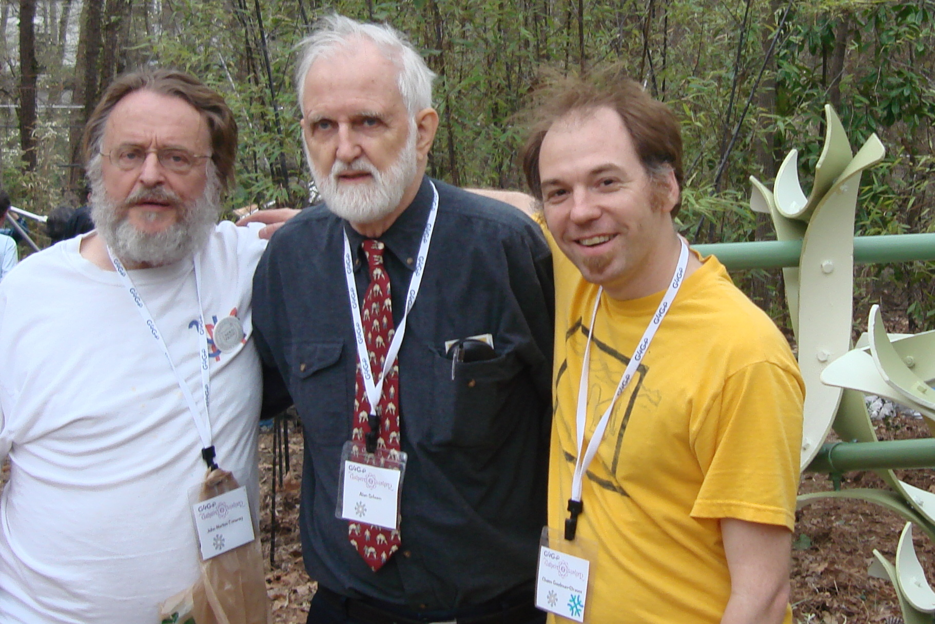
by a phone call from
Tom Rodgers,
the Atlanta impresario who founded — and continues to host — the
now binennial Gatherings for Gardner.
Tom told me that he had seen ceramic versions of d7 rhombic tilings on the
Saxe-Patterson
website and wanted to use such a design as a logo for G4G7.
After Tom's call, I decided to take up cutting and pasting again. Here's what the tiling looks like now:

Fig. C3.17.2
The completed (0,0,1)B-3 paste-up
When I examined the unfinished panel,
it suggested some
mathematical questions that I probably hadn't thought much about in 1981 but
that now seemed to demand answers.
I've since found answers for most — but not all — of these questions.
Many of the questions and answers are discussed in § C3.1-C3.8.
The most awkward of these questions is how to prove that as the pattern grows radially outward, it can retain the
d7 symmetry of the central nucleus (core) at every stage of recursion,
i.e., that a proper wedge exists at every stage (cf.§ C3.1 and § C3.10).
I still can't answer this question,
but at least it can now be said (cf.§ C3.4 and § C3.8) that for both pointed and blunt tilings,
(a) the d7-symmetric
necklaces that decorate the heptagonal boundary mirrors
can be constructed at every stage of recursion, and
(b) for prime n the composition of every necklace is unique.
In practice it hardly matters
whether one can prove that a tiling can be extended symmetrically outward forever,
since the tiling expands so rapidly at each stage that
it is unrealistic to consider physical tilings (or even mere computer images!)
that exceed four or five stages.The precise number
of stages depends, of course, on whether
you're planning to cover just the floor of a room or
an area the size of Rhode Island.
RP7 tilings are in a very rough sense self-similar centro-symmetric tilings
of the Euclidean plane by rhombs.
The three prototile rhombs of RP7 tilings are unmarked, and there are
no matching rules.
The two prototile rhombs of Penrose tilings,
by contrast, are marked
in such a way as to prevent periodic tilings
and allow only aperiodic tilings,
when Penrose's matching rules are imposed on the marked tiles.
Although there is a superficial connection between RP7 tilings and
the two most symmetrical examples of Penrose tilings,
the d5-symmetric SUN and STAR,
none of the subtle features of Penrose tilings are found in RP7 tilings.
These features include:
(a) quasiperiodicity,
which implies Conway's town theorem ('local isomorphism'),
(b) projection from a five-dimensional cubic honeycomb,
(c) a basis for mathematical modeling of the 3-dimensional
quasicrystals
discovered by Dan Shechtman and his collaborators in 1984,
(d) the dual relationship
between the rhombs of a tiling and the vertices of a de Bruijn pentagrid,
(e) derivation by the inflation
of a finite tiling,
(f) matching rules
for kite/dart tilings and tilings by rhombs,
(g) ubiquitous role of the
golden ratio and Fibonacci sequences,
etc.
C3.18 Stereoscopic view of (1,0,0)B stepped pyramid
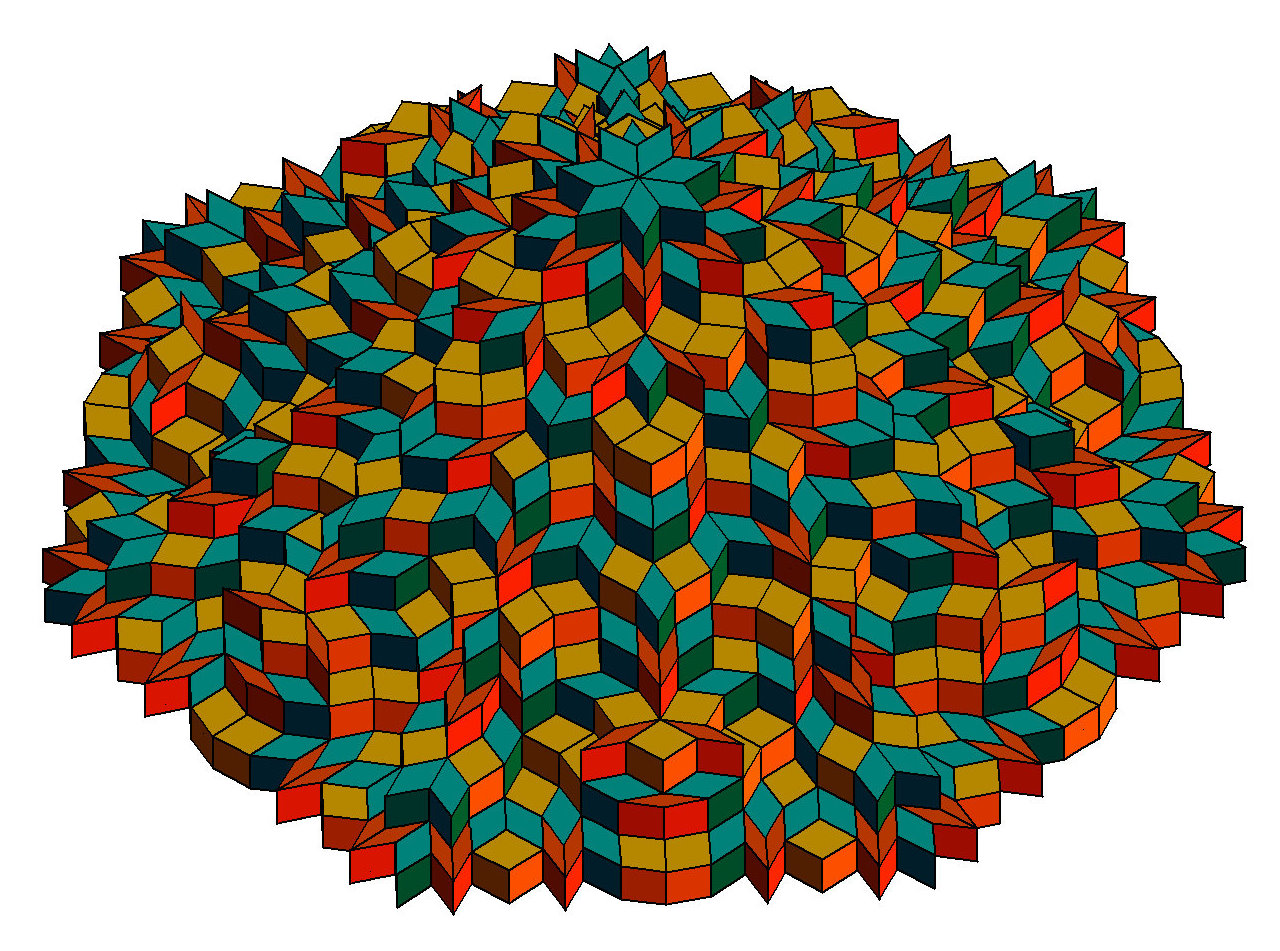

Fig. C3.18.1
cross-eyed stereoscopic view of the (1,0,0)B tiling
transformed into a stepped pyramid
C4. Rhombic wallpaper (periodic tilings derived from a variant form of de Bruijn multigrids)
- C4.0 Introduction
- The trivial examples derived from regular and uniform tilings
- How densely can rosettes be embedded?
- Adaptation of the Gessel and de Bruijn algorithms
- The six rosettes for n = 5
- Single-lattice and poly-lattice tilings
- Lattice stars
- The classes and types of RW tilings
- Superdense, dense, and sparse tilings
- Examples of straight row tiling lattice stars
4.5
- C4.1 Straight row tilings, aligned: even n
- C4.2 Straight row tilings, aligned: odd n
- C4.3 Straight row tilings, staggered: even n
- C4.4 Straight row tilings, staggered: odd n
- C4.5 Zig-zag row tilings: odd n
- C4.6 Square lattice tilings: even n
- C4.7 Square lattice tilings: odd n
- C4.8 Rectangular lattice tilings: even n
- C4.9 Hexagonal lattice tilings: even n
- C4.10 Hexagonal lattice tilings: odd n
- C4.11 Additional examples of RWn
- C4.12 How to construct a RWn
- C4.13 Origins of RWn
C4.0 Introduction
Using the n(n − 1)/2 rhombs of SRIn as prototiles, it's easy to
construct examples of periodic tilings in which there are
no embedded rosettes (aside from the rosette
composed of a single square when n is even).
Here is an example of such a tiling for n = 7:
Fig. C4.0.1
Periodic tiling for n = 7 in which
there are no embedded rosettes
I will ignore all such tilings, and
I'll call periodic tilings by the
rhombs of SRIn in which rosettes of order n are embedded
rhombic wallpaper (or RW) of order n.
For n = 2, 3, 4, and 6, there exist RW tilings that I call
the trivial examples. They are based on
two of the three regular tilings:
4.4.4.4, tiled by squares,
6.6.6, tiled by hexagons,
and on
two of the eleven
uniform tilings:
4.8.8, tiled by squares and octagons and
4.6.12, tiled by squares, hexagons, and 12-gons.
Figs. C4.0.1 a and b
Figs. C4.0.2 a and b
Figs. C4.0.3 a and b
Figs. C4.0.4 a and b
Four regular and uniform tesselations (left)
and the four trivial examples of RW tilings based on them (right)
Now consider the following admittedly frivolous question:
How densely can non-overlapping rosettes of order n be embedded in a RW tiling of order n?
This question is related to a slightly more restricted one:
Imagine an infinite orchard of identical trees arranged on a square lattice.
Let ρtree = the tree density (number of trees per unit area).
A straight cable is stretched from each tree to 2n other trees,
which are called its 'connected neighbors'.
Each cable is incident at no tree other than the two at its ends.
The arrangement of the 2n connected neighbors ('connected-neighbor
configuration') is identical, up to rotation about a vertical axis, for all trees.
The number of distinct crossed pairs of cables ('nodes') at each point
at which m cables cross is equal to m(m − 1)/2.
Let ρnode = the node density (total number of
crossed cable pairs per unit area of the rhombic tiling dual to the set of nodes),
and call the ratio ρnode/ρtree
the tree-normalized node density.
For given n, which periodic orchard and connected-neighbor configuration have the smallest
tree-normalized node density?
This orchard model is a paraphrase of the 'star grid' scheme for
generating RW tilings that is described below.
In the first three of the four examples shown above (Figs. C4.0.1b-C4.0.3b), the rosettes of order n
have maximal density,
i.e., they occupy the largest possible fraction of the tiling area
among all RW tilings of the same order.
But the density of the tiling for n = 6 in Fig. C4.0.4b
is almost seven percent less than that of the kagome tiling
in Fig. C4.0.5, which is conjectured to have maximal density.
Fig. C4.0.5
density = (8√ 3 − 12)/3 ≅ .618802
For small n, there are a few empirical rules — described below — that
predict which RW tiling has maximal density.
For every n>2, there is an uncountable infinity of RW tilings in which the
density of the rosettes of order n is less than maximal.
I describe below a systematic procedure, adapted from
Gessel's algorithm for rosettes and from
de Bruijn's multigrid algorithm
for aperiodic tilings,
for generating RW tilings of both maximal and sub-maximal density.
For n ≠ 2, the density can be made arbitrarily close to any
value less than or equal to the maximal density, by using the splitting and augmenting
operation illustrated in § 4.8.
* * * * *
(For a concise description of de Bruijn's multigrid algorithm,
see pp. 33-44 of Laura Effinger-Dean's undergraduate
honors thesis.
The original article by de Bruijn is entitled
"Algebraic theory of Penrose's non-periodic tilings of the plane",
Nederl. Akad. Wetensch. Proceedings Ser. A 84 (Indagationes Math. 43)
(1981) 38-66.
It was reprinted in The Physics of Quasicrystals, ed. P.J. Steinhardt and
S. Ostlund, World Scientific Publ. Comp., Singapore (1987), pp. 673-700.)
* * * * *
In any aperiodic tiling for n ≥ 3 that is the
dual of a de Bruijn multigrid,
one cannot help noticing the not necessarily symmetrical rosettes of order
n that are embedded here and there.
(Here is an example for n = 7.)
The occurrence of rosettes is statistically inevitable in these aperiodic tilings.
A rosette is the dual of the k(k − 1)/2 points of
intersection of any set of k lines in which each line
intersects every other at a unique point.
In every de Bruijn pentagrid, arrangements of five lines
that satisy this condition occur infinitely often, since Conway's
town theorem guarantees that the portion P of the tiling dual to every such arrangement is
no farther from its nearest replica than slightly more than
twice the diameter of P.
Here is an example of one of the six five-line arrangements in a pentagrid:
Fig. C4.0.6
Ten points in a de Bruijn pentagrid
that are dual to a rosette of order 5
These six line arrangements define the following six rosettes:
Fig. C4.0.7
The six rosettes for n = 5
For n > 5, without analogs of Conway's n = 5 town theorem
we don't have an upper bound on the distance between a rosette that is
embedded in a de Bruijn aperiodic tiling and its nearest replica.
(Incidentally, for n > 5, the number of ways a rosette of order n
can be tiled by the rhombs of
SRIn is unknown. But I have found that for n = 6,
this number is at least 49.)
The scheme I have devised to explore the rosette density problem
for n ≥ 3 can be used to create an uncountable infinity of RW tilings
containing embedded rosettes of order n.
It generates a 'star grid' from one or more 'lattice stars'. Every intersection
of two lines of the star grid is the dual of a rhomb
in a RW tiling.
I'll first describe the scheme for single-lattice tilings,
in which a rosette of order n is centered at every lattice point of the tiling.
There are no other such rosettes in the lattice fundamental domain.
Then I will describe the version for poly-lattice tilings,
in which a rosette of order n is centered
at each of m points (m>1) in
the lattice fundamental domain. In this case, the rosettes are centered at the lattice points of
m congruent sub-lattices of the tiling. (The kagome tiling in Fig. C4.0.5 is an
example of a poly-lattice tiling with m = 2.)
Scheme for single-lattice tilings
(i) Choose a lattice L.
(ii) Construct a lattice star composed of 2n distinct rays
(line segments), each of which extends from a common root-lattice point P0
to a terminal lattice point Pk (k = 1, 2, ..., 2n).
The 2n terminal lattice points are all distinct.
(iii) Generate a star grid by translating the lattice star
to each lattice point of L.
The rhombs of the tiling are dual to the vertices of the star grid.
Scheme for poly-lattice tilings (m congruent sub-lattices)
(i) Choose a lattice L.
(ii) Construct m lattice stars—one for each of
m sub-lattices Lk (k = 1, 2, ...,
m) congruent to L, each composed of 2n distinct rays.
In each lattice star, every ray extends from a common root-lattice point P0
to a terminal lattice point Pk
(k = 1, 2, ..., 2n), which may belong either to the same
sub-lattice or to a different sub-lattice. The 2n terminal lattice
points are all distinct.
(iii) Generate a star grid by translating the lattice star for each
sub-lattice Lk
to every other point of Lk.
The rhombs of the tiling are dual to the vertices of the star grid.
For the unit square lattice (integer lattice),
we define the magnitude of a lattice star — using the conventions of
taxicab geometry — as the sum of
the 'manhattan lengths' of the 2n rays of the star.
By this measure, the lattice star in Fig. C4.0.8, for example, has magnitude 44.
Fig. C4.0.8
Star magnitude = 44
For RW tilings for small n on either square or rectangular lattices,
rosette density and star magnitude are found to be inversely correlated.
Examples are shown in § 4.8. When two different lattice stars for the same n
have the same magnitude, the rosette density is usually found to be
larger in the tiling for which the tree-normalized node density
in the star grid is smaller.
(If the tree-normalized node density were replaced by a weighted count of nodes,
each weight being the area of the rhomb dual to each node, then the
tree-normalized node density would be exactly inversely correlated.)
It is convenient to identify RW tilings of order n by class and type.
These terms are defined below. Tilings are ranked according to density as follows:
1. A tiling with the highest density of any tiling
of order n is called
superdense.
2. A tiling with the highest density of any tiling
of order n of its type is called
dense.
3. A tiling with density less than the highest density
of any tiling of order n of its type is called
sparse.
The tilings for n = 2 and n = 3 in Figs. C4.0.1b and C4.0.2b, respectively,
are superdense, since their density is equal to 1.
The tiling for n = 4 in Fig. C4.0.3b
is superdense. Its density is equal to 2 (√ 2 − 1) ≅ .828427,
which is maximal. (It is easily proved that there exists no tiling by regular octagons
with higher density.)
The tiling for n = 6 in Fig. C4.0.4b is
sparse,
since its density of 1/√ 3 ≅ .577350 is
less than the density (8√ 3 − 12)/3 ≅ .618802 of the kagome
tiling, shown in Fig. C4.0.5, which is conjectured to be superdense.
Although all of the tilings for n<9 conjectured to be superdense
have reflection symmetries, the tiling for n = 9 (cf. Figs. C5.9.1a and b)
that is conjectured to be superdense does not — it has only p3 symmetry.
Its density is almost 30% larger than that of the tiling with p3m1 symmetry in Fig. C4.10.2.
Every RW tiling treated here is characterized as belonging to either the row class or the dispersed class.
Within the row class, there are two sub-classes: straight and zig-zag.
Within each of these two sub-classes, there are four types.
Within the dispersed class, there are three sub-classes: square lattice,
hexagonal lattice, and other lattices.
This classification scheme is by no means exhaustive.
The kagome tiling in Fig. C4.0.5 belongs to neither dispersed nor row class.
Neither do tilings in which all the rosettes are arranged in closed rings, with every
rosette incident at each of two neighbors.
In another example, some rosettes are incident
at no other rosettes, and still other rosettes are arranged in rows.
I have not investigated examples of every one of the types listed below.
Except for a few small values of n, I have not proved
maximal density. The labels 'dense' and 'superdense' should be regarded as tentative
except where stated otherwise.
THE CLASSES, SUB-CLASSES, AND TYPES OF RHOMBIC WALLPAPER TILINGS
- Row tiling
- The rosettes are arranged in parallel rows.
Every rosette is contiguous to exactly two other rosettes in the same row.
No rosette shares a vertex with a rosette in another row.
- Straight row
- The rosette centers lie at equal intervals on a straight line.
- Vertex-sharing
- Contiguous rosettes share a vertex, but not an edge.
- Edge-sharing
- Contiguous rosettes share an edge.
- Aligned
- The line between the centers of two contiguous rosettes
is perpendicular to the line between the center of either of them and the
center of the nearest rosette in an adjacent row.
- Staggered
- Non-aligned
- Zig-zag
- The rosette centers lie at the vertices of a symmetrical sawtooth.
- Vertex-sharing
- Contiguous rosettes share a vertex, but not an edge.
- Edge-sharing
- Contiguous rosettes share an edge.
- Aligned
- The line between the centers of two contiguous rosettes
is perpendicular to the line between the center of either of them and the
center of the nearest rosette in an adjacent row.
- Staggered
- Non-aligned
- Dispersed tiling
- No two rosettes are contiguous
- Square lattice
- Hexagonal lattice
- Other lattices
A RW tiling may also be categorized according to the residue class of
n, e.g., even, odd, congruent to 3 (mod 6), etc.
For every tiling, whether it is of the
dispersed or row class, the wallpaper group is identified.
But at every point of intersection of three or more lines in a star grid,
the orientation in the tiling plane and — for
four or more intersecting lines —
the symmetry of the arrangement of rhombs
inside the convex polygon ('oval')
dual to the point of intersection is indeterminate. An arbitrary choice
of orientation (and also of symmetry, when four or more lines are involved) must be made in each such case.
The wallpaper group of the tiling depends on precisely which choices are made.
For some families of dense tilings of a particular type that are
parametrized by the order n of the tiling,
the dependence of density on n — for small n — can be described
by an algebraic expression conjectured to hold for all n.
In some cases, it is not difficult to guess an asymptotic form for this expression
that is confirmed by numerical calculations,
but I have not proved any of these results. Some of these asymptotic expressions appear following Fig. C4.10.2.
EXAMPLES
Let's now examine examples of tilings of several types,
in increasing order of n.
The tiles are defined to have unit edge length.
In several cases, I have included the lattice star or star grid (or both).
In addition to density ρn, I record the wallpaper group and — for
row tilings — λn, the
distance between the center-lines of adjacent rows.
Some types have no representatives, because I am considering only edge-to-edge tilings,
i.e., tilings in which the corners and sides of the tiles coincide
with vertices and edges of the tiling (cf. Tilings and Patterns, by Grunbaum
and Shephard, p. 18).

Fig. C4.0.9
Examples of straight row tiling lattice stars for small n.
Top row: lattice stars for the square lattice.
Bottom row: lattice stars for the hexagonal lattice.
C4.1 Straight row tilings, aligned: even n
Fig. C4.1.1
n = 2
Fig. C4.1.2
n = 4
Fig. C4.1.3
n = 6
Fig. C4.1.4a
n = 8
Straight row aligned edge-sharing
ρ8 ≅ .394591
λ8 ≅ 10.1371
pmm
(This is the same tiling as the one at the right in Fig. C4.1.6.)
Fig. C4.1.4b
n = 8
Lattice star for the tiling of Fig. C4.1.4a
Fig. C4.1.4c
n = 8
Star grid for the tiling of Fig. C4.1.4a
(This star grid is drawn on the same scale as the lattice star in Fig. C4.1.4b.)
Fig. C4.1.5a
n = 8
Straight row aligned vertex-sharing
ρ8 ≅ .253965
λ8 ≅ 15.4476
pmm
(This is the same tiling as the one in Fig. C4.1.5d
and is a slightly rearranged version of the tiling at the left in Fig. C4.1.6.)
Figs. C4.1.5b and C4.1.5d demonstrate that although the angular distribution
of the 2n rays in a lattice star is not uniform,
those rays represent 2n radial lines that are uniformly distributed:
each side of every rhomb in the tiling is perpendicular to one of the two
radial lines associated with the pair of intersecting
rays whose intersection is dual to the rhomb.
Fig. C4.1.5b
n = 8
Lattice star for the tiling of Fig. C4.1.5a
Fig. C4.1.5c
n = 8
Star grid for the tiling of Fig. C4.1.5a
(This star grid is drawn on the same scale as the lattice star in Fig. C4.1.5b.)
Fig. C4.1.5d
n = 8
Straight row aligned vertex-sharing
Ladders 0 (red), 1 (green), 2 (blue), 3 (violet)
(cf. rays 0, 1, 2, 3 in the lattice star of Fig. C4.1.5b)
Each thick black radial segment in the central rosette is
perpendicular to the rungs of its associated ladder.
Fig. C4.1.6
n = 8
Fig. C4.1.7
n = 10
C4.2 Straight row tilings, aligned: odd n
Fig. C4.2.1
n = 3
ρ3 ≅ .75000
λ3 ≅ √ 3
pmm
Fig. C4.2.2
n = 5
ρ5 ≅ .5414
ρ5 ≅ .5150
λ5 ≅ 4.9798
λ5 ≅ 4.8541
pmm
Fig. C4.2.3
n = 7
ρ7 ≅ .3466
ρ7 ≅ .3745
λ7 ≅ 9.8447
λ7 ≅ 9.3488
pmm
C4.3 Straight row tilings, staggered: even n
Fig. C4.3.1
n = 2

Fig. C4.3.2
n = 4
Fig. C4.3.3
n = 6
Fig. C4.3.4
n = 8
C4.4 Straight row tilings, staggered: odd n
Fig. C4.4.1
n = 3
ρ3 ≅ 1
λ3 ≅ 1.5
pmm
Fig. C4.4.2
n = 5
ρ5 = (1 - 8√ 5)[25 - 10√(6 - 2√ 5)] ≅ .669153
λ5 ≅ √ 5 + 1.5 ≅ 3.7361
pmm
Fig. C4.4.3
n = 7
ρ7 ≅ .460658
λ7 ≅ 7.5978
pmm
C4.5 Zig-zag row tilings, aligned: odd n
Fig. C4.5.1a
n = 5
Lattice star for sites of type A in zigzag-row tiling of Fig. C4.5.1d.
A and B are the two inequivalent types of sites in each lattice fundamental domain.

Fig. C4.5.1b
n = 5
Lattice star for sites of type B in zigzag-row tiling of Fig. C4.5.1d.
A and B are the two inequivalent types of sites in each lattice fundamental domain.
Fig. C4.5.1c
n = 5
Star grid for the zigzag-row tiling of Fig. C4.5.1d
(This star grid is drawn on the same scale as the lattice stars in Figs. C4.5.1a and b.)
Fig. C4.5.1d
n = 5
Zigzag-row tiling
ρ5 = 5 − 2√ 5 ≅ .527864
λ5 ≅ 4.9798
(Skeletons of zig-zag rows of non-overlapping rosettes)
In Figs. C4.5.2 and C4.5.3 are two zig-zag row tilings for n = 7.
Each of them is a poly-lattice tiling, with m = 2.
Fig. C4.5.2a
n = 7
Lattice stars A and B for zigzag-row tiling no. 1 of Fig. C4.5.2c
Fig. C4.5.2b
n = 7
Star grid for zigzag-row tiling no. 1 of Fig. C4.5.2c
Fig. C4.5.2c
n = 7
Zigzag-row tiling no. 1
ρ7 ≅ .4655
λ7 ≅ 7.8948

Fig. C4.5.3a
n = 7
Lattice stars A and B for zigzag-row tiling no. 2 of Fig. C4.5.3c
Fig. C4.5.3b
n = 7
Star grid for zigzag-row tiling no. 2 of Fig. C4.5.3c
Fig. C4.5.3c
n = 7
Zigzag-row tiling no. 2
ρ7 ≅ .4547
λ7 ≅ 8.5429
Now let us look at some examples of lattice tilings — mostly, but not
all — dense tilings. We begin with
C4.6 Square lattice tilings: even n
Fig. C4.6.1
n = 4
ρ4 = 2 (√ 2 − 1) ≅ .828427
Fig. C4.6.2
n = 4
ρ4 = 2 (√ 2 − 1) ≅ .828427
Fig. C4.6.3
n = 4
ρ4 = 2 (√ 2 − 1) ≅ .828427
Fig. C4.6.4a
n = 8
If you fill these 81 holes (and half-holes) ...
Fig. C4.6.4b
n = 8
with these 81 polka dots ...
Fig. C4.6.4c
n = 8
you get this superdense tiling.
ρ8 ≅ .425442
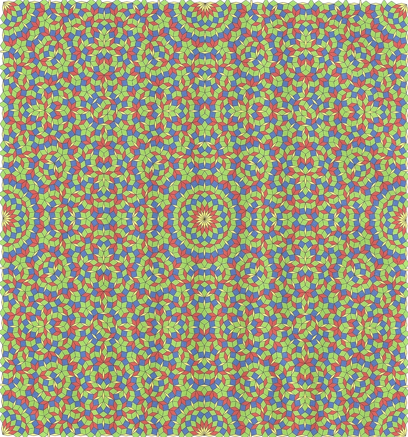
Fig. C4.6.5
n = 8
ρ8 ≅ .0143164
Compare this quite sparse tiling
to the superdense tiling in Fig. C4.6.4c.
(To see this one in brighter colors, look
here.)
Fig. C4.6.6a
n = 10
ρ10 ≅ .226550
Introducing a non-convex prototile into this tiling, which has no reflection symmetries,
changes it into the one shown in Fig. C4.6.6b, which does have reflection symmetries.
Fig. C4.6.6b
n = 10
This tiling has reflection symmetries
and a translational fundamental domain only half as large as in Fig. C4.6.6a.
Fig. C4.6.7
n = 12
ρ12 ≅ .261899
For a pdf version of this tiling, look
here.
In addition to the very prominent d3 rosettes of order 12,
smaller rosettes of orders 3, 4, and 6 appear
in this pattern.
You can count a total of sixteen rosettes in each translational fundamental region
of the lattice.
(The symmetry of this tiling is reduced by errors in the
orientation of the rosettes.)
C4.7 Square lattice tilings: odd n
C4.8 Rectangular lattice tilings: even n
Fig. C4.8.1a
n = 8
Lattice star for rectangular lattice tiling in Fig. C4.8.1c
Star magnitude = 52
Fig. C4.8.1b
n = 8
Star grid for rectangular lattice tiling in Fig. C4.8.1c
Fig. C4.8.1c
n = 8
Star magnitude = 52
Fig. C4.8.2a
n = 8
Lattice star for rectangular lattice tiling in Fig. C4.8.2c
Star magnitude = 44
Fig. C4.8.2b
n = 8
Star grid for rectangular lattice tiling in Fig. C4.8.2c
.gif)
Fig. C4.8.2c
n = 8
Star magnitude = 44
_split.gif)
_expanded.gif)
Fig. C4.8.3
n = 8
Splitting (left) and augmenting (right) the tiling in Fig. C4.8.2c
_tiling.gif)
Fig. C4.8.4a
n = 8
Lattice star for rectangular lattice tiling in Fig. C4.8.4c
Star magnitude = 44
_tiling.gif)
Fig. C4.8.4b
n = 8
Star grid for rectangular lattice tiling in Fig. C4.8.4c
_rect_lattice.gif)
Fig. C4.8.4c
n = 8
Star magnitude = 44

Fig. C4.8.5a
n = 8
Star magnitude = 36
Fig. C4.8.5b
n = 8
C4.9 Hexagonal lattice tilings: even n
.gif)
Fig. C4.9.1
n = 6
ρ6 =1/√ 3 ≅ .577350
superdense
C4.10 Hexagonal lattice tilings: odd n
Fig. C4.10.1a
n = 9
ρ9 ≅ .341644
superdense
p3
.gif)
Fig. C4.10.1b
(Another coloring of the superdense tiling of Fig. C4.10.1a)
Fig. C4.10.2
n = 9
ρ9 ≅ .263346
sparse
p3m1
Below are:
C4.11 Additional examples of RWn
C4.12 How to construct a RWn
C4.13 Origins of RWn
C4.11 Additional examples of RWn
Below are examples of both dense and sparse RWn tilings
for n in the interval [2,22].
In many of the the RW tilings shown here,
each shape of rhomb has a characteristic color (or shading).
Some color schemes
produce striking subliminal patterns—approximations of
circles, triangles, hexagons, etc.
The scale of such patterns is sometimes so large that
an assembly of several unit cells of the tiling may be required to reveal them.
It is characteristic of RWn tilings that
along lines of reflection of the tiling lie infinite linear strings of rhombs
that are analogs of minimal pointed beadstrings
(cf. § C3.2): each bead is composed of a single rhomb.
Some tilings in addition contain finite strings composed of blunt beads, aligned in directions
that do not coincide with lines of reflection of the tiling.
RW21(4) is an instructive example.
The axes of three pointed strings of infinite length,
intersecting at the center of the image, lie on
lines of reflection of the tiling at 0, 60, and 120 degrees from the vertical.
In addition every pair of nearest neighbor rosettes is joined by a finite string of blunt beads.
These blunt strings can only partially mimic the mirroring effects of blunt beadstrings in RPn tilings,
described in § 3.2 and § 3.3. The tiling would be perfectly symmetrical by reflection
in the longitudinal axis of each such blunt string if it were not for the fact that neither
(a) the arrangement of rhombs in the interior of the beads of each string
nor
(b) the tiling of the rosettes
is symmetrical by reflection in those axes.
In RW21(4), the rosettes would require
d6 symmetry, but symmetry of even order is impossible for rosettes (cf. § B1).
RW9, illustrates the same effects.
n = 2: Regular tiling by squares (square lattice)
n = 3: Regular tiling by hexagons,
each tiled by three congruent rhombs (hexagonal lattice)
RW6(1)
n = 7: Not every rosette is centered at a lattice point (rectangular lattice).
Fig. C4.11.1
RW7(1)
ρ7 ≅ 0.5289856
I will soon post a picture of the 25" x 38" RHOMBBURST poster,
which includes an article at the bottom summarizing the state of knowledge in 1995 about Penrose tilings.
Unlike RW8(2) (above), the tiling of the
RHOMBBURST poster is not a wallpaper pattern—it is a centro-symmetric
tiling with a single center of symmetry.
It has 16 lines of reflection
and therefore has d16 symmetry. How many lines of reflection do you find in a unit cell
(fundamental domain under translation) of
the periodic RW8(2) (above)?
RW9(1)
is a more colorful version of RW9.
Note that the image is rotated, relative to RW9, by one-sixth of a turn around its center.
In this orientation, it is symmetrical by reflection in a vertical line through the center.
RW10(1) is a row tiling.

Fig. C4.11.2
Two colorings of RW10(1)
For other images of RW10(1), see
RW10(2) ,
RW10(3)
or
RW10(4) .
Note that exactly halfway between adjacent
rows of large rosettes in RW10(1), there is a string of strawberry rosettes of
order 5. In row tilings of odd order,
there is a medial string of convex polygons, in a regular
alternating sequence, with n-1 and n+1 sides, respectively.
I will soon add an example or two.
In RW10(1), the large rosettes in
adjacent rows are 'staggered' (offset) by a
rosette circumradius.
There also exist 'non-staggered'
row tilings, for both odd and even n.
In row tilings,
the convex 'wave fronts' of tiles that border
large rosettes in one row are transformed
into concave 'wave fronts'
by the time they reach the large rosettes in an adjacent row.
I call the pattern elements that mediate this change
ginkgo leaves.
RW16_row and
RW22_row demonstrate
the hierarchical arrangement of ginkgo leaves in row tilings.
Ginkgo leaves bear a superficial resemblance to
the arbelos (shoemaker's knife) of Archimedes, but while
the circular arcs that define the
boundary of the arbelos do not all have the same curvature,
all three boundary 'curves' of a ginkgo leaf
have the same curvature.
n=15: RW15 has a hexagonal lattice.
Fig. C4.11.3
RW15
For a pdf version, look
here.
RW15(1)
is another coloring of RW15.
n=16: RW16(1) illustrates how
broken symmetries unavoidably appear when you embed a rosette—which
necessarily has symmetry of odd order—in a
RW tiling with no symmetries of odd order.
(In its present form, this tiling has no symmetries,
but a half-turn rotation of every rosette in alternate horizontal rows
would introduce horizontal lines of reflection.)
In RW16_row, a row of n=8 small rosettes lies
halfway between each pair of adjacent rows of n=16 large rosettes:
Fig. C4.11.4
RW16_row
The horizontal center-line of each row of n=16 rosettes
is a line of reflection, but
the horizontal center-line of each row of n=8 rosettes
is not a line of reflection.
The enlarged image below shows that the 16-gon boundaries of adjacent n=8 rosettes
are oppositely rotated around their centers.
Fig. C4.11.5
Adjacent n = 8 rosetttes in RW16_row are oppositely rotated.
n=21: RW21(1)
is an ambitious example of a
RWn tiling. To see the smallest rhomb clearly,
you may have to enlarge the image.
It's apparent that d3 rosettes fit more harmoniously
on a hexagonal lattice
than on a square lattice.
I'll explain below how the overall symmetry
is affected by the parity — (even n vs. odd n) — of the
SRIn.
To see how color choices for the rhombs affect RW21, see
RW21(2),
RW21(3),
RW21(4),
RW21(5), and
RW21(6).
RW21(6)
is a monstrously large piece of RW21.
It contains seven times as many rhombs as the other versions.
I didn't attempt to find color choices that would emphasize 'subliminal'
image effects, but you can see suggestions of such effects
in the roughly circular 'watermarks' embedded in the pattern.
Here
is an ordered sequence of ten images of RW21. In each image only one shape of
rhomb is highlighted. The sequence begins with the smallest
rhomb and ends with the largest rhomb.
By closely examining image sets like these, one could probably
discover how to enhance the strength of particular subliminal images.
(I have no plans to do that!)
n=22: RW22 is
a row tiling of order 22 that shows the 'mortar' between rosettes
but not the rosettes themselves.
C4.12 How to construct a RWn
Let's first recall that a de Bruijn multigrid is
a set of n overlapping uniformly rotated grids of parallel lines. Here's an example for n = 5:
Fig. C4.12.1
A de Bruijn pentagrid
If no point of a multigrid belongs to more than two of its n grids,
de Bruijn calls the multigrid regular;
otherwise he calls it singular.
A star grid of order n is the periodic counterpart of a de Bruijn multigrid of order n.
DEFINITIONS:
(1) A lattice star of order n is a set of 2n rays (line segments)
associated with the lattice L.
One end of every ray is incident at the common lattice point P0;
the other end is incident at a distinct one of the
lattice points Pk (k=0, 1, 2, ..., n-1).
The 2n rays of the lattice star are labelled CCW
by their n integer indices
0, 1, 2, ..., n, n+1, ..., n+2, ..., 2n-1 (mod n).
A lattice star has the same point symmetry as its root lattice point P0.
(2) A star grid of order n
is the union of congruent parallel lattice stars of order n,
one specimen of which is rooted at every point of the lattice L.
In a star grid of order n, n lines intersect
at every lattice point.
Mimicking de Bruijn, we call any point of a star grid at which only
two lines intersect a regular point, and any point at which
more than two lines intersect a singular point.
The dual of every regular point in a star grid is a rhomb
whose face angles are defined by the difference between the indices
of the two rays that intersect there.
The set of rhombs dual to a singular point at which m lines intersect
(m=3, 4,...,n) is a convex assembly of m(m-1)/2
rhombs that tile a 2m-gon.
The precise arrangement of these rhombs is indeterminate.
It is appropriate, whenever possible, to arrange them in a tiling of the 2k-gon
that has the point symmetry of the singular point.
If the point symmetry of the singular point is dihedral of odd order,
it is always possible to find an arrangement of these rhombs with the same symmetry.
But if the point symmetry of the singular point is dihedral of even order,
there exists no arrangement of the rhombs with the same symmetry.
For these reasons, RWn tilings of odd order
are somewhat more 'harmonious' in appearance than those of even order —
their space group is likely to contain more symmetries.
For large separation of the rosettes (sparse dot packing) in a RWn tiling,
the unit cell of the lattice is large, and the tiling may at first seem
indistinguishable from a pseudo-Penrose tiling derived from
a de Bruijn multigrid (cf. de Bruijn 2/14(1), for example).
A lattice star for n=9 is shown below. Because this lattice star produces
a RW9 tiling with higher density than any alternative
set of lattice points of the same symmetry, it is called dense.
For illustration purposes, circles have been centered at each lattice point to indicate the positions (although
not the sizes) of the rosettes.
In the associated star grid, nine lines intersect at the center of every circle.
These lines are truncated here
by the circle boundaries.
Fig. C4.12.2
Fig. C4.12.3
This extremal star grid for n = 9 is
a periodic array of replicas of the lattice star in Fig. C4.12.2.
The dual of this star grid is the tiling in
Fig. C4.10.2,
which is shown in color
here.
(Note that a chain of three-bead Conway worm segments connects each pair of nearest-neighbor rosettes.)
It is instructive to compare an edge between a particular pair of lattice points
in the star grid with the corresponding chain of rhombs in the tiling.
In the star grid above, there are only two kinds of edges—those between nearest-neighbor dots
and those between fourth-nearest-neighbor dots.
Choose a particular edge and then
follow the chain of rhombs ('ladder' with parallel rungs) between
the two rosettes in RW9(1) that correspond to the
pair of lattice points joined by the edge.
Fig. C4.12.4
An extremal star grid for n = 15,
which is the dual of the tiling RW15(1).
Fig. C4.12.5
A zoom shot of the region just below the center of the image in Fig. C4.12.4
Fig. C4.12.6
A single lattice unit cell of the extremal star grid for n = 16,
which is the dual of
RW16(1)
 .
.
Fig. C4.12.7
The lattice star for the extremal tiling RW21(1).
 .
.
Fig. C4.12.8
Star grid for the extremal tiling RW21(1)
The star grid is a superposition of the lattice stars in Fig. C4.12.7.
(Lattice points here are approximately six times farther apart than in Fig. C4.12.7.)
C4.13 Origins of RWn
In 1991, in the first edition of the manual for the tiling puzzle ROMBIX
,
I posed a special puzzle challenge called 'POLKA DOTS'. It is reformulated here as
a puzzle for RWn.
Suppose you are required to tile a vast flat area—like the state of
Rhode Island, for example—with Rhombic Wallpaper.
Suppose further that there are rosettes ('dots') embedded in this tiling.
All of the spaces (the 'mortar') between the dots must be tiled by
the rhombs of RWn.
HOW DENSELY CAN YOU PACK THE 'DOTS'?
I'll call this rather messy problem
connecting the dots.
It's an example of a so-called extremal problem.
In 1991 I didn't have a general solution
and I still don't have one. For n = 2, 3, and 4, the problem is trivial,
because solutions follow immediately from properties of
regular and semi-regular tilings of the plane
by squares, hexagons, and octagons.
When I revisited this problem in 2002, I replaced the rombiks of order eight
by the rhombs of SRIn.
Perhaps I was guided by what Halmos called "Polya's dictum":
"If you can't solve a problem, then there is an
easier problem you can't solve—find it!"
I don't know whether the solution for every n is a periodic tiling,
but if it is, then it can be found from
an algorithm I adapted from the
Gessel-de Bruijn method of
associating rhombs with their duals—the points of intersection in configurations of lines.
The algorithm makes it possible to investigate candidate solutions
for any particular n by using a periodic variant of
the multigrids invented by de Bruijn for his
analysis of Penrose tilings.
I call these modified grids star grids.
I examined not only dense dot packings,
but also sparse ones
in which the rosettes are quite widely separated.
The density of the rosettes in a tiling ('density') is determined by the
design of its lattice star—the basic structural unit
of the star grid dual of the tiling. Star grids and lattice stars are defined below.
For a partial summary of results obtained so far, see dot spacing data.
These results have been confirmed for small values of n, but they have not yet been proved.
Back to GEOMETRY GARRET


grid.gif)

 ,
,